arXiv/viXra - Embeddings

Note: The Jupyter/Colab notebooks relevant to this post are here on my GitHub page. My vectorized pytorch_lightning GloVe implementation considered in this post can be found here.

Language Learning

The models I have considered up to this point have been purely trained on the task of distinguishing arXiv and viXra papers. Though the recurrent architectures detailed here have some awareness of the positional relations between the words in the relevant text, I have not specifically attempted to attune them to the patterns inherent in language.

Models view the world fairly myopically, with a single-minded focus on the training objective. For instance, though the recurrent architectures do a reasonable job of distinguishing arXiv from viXra, one would expect them to perform poorly if asked to transfer their knowledge to tasks such as clustering semantically related words together or predicting the next word in a title, given all preceding words. I would not expect them to have learned much meaningful information about the structure of language.

Natural Language Processing (NLP) models can benefit greatly from the reversed process: first train a base model on a fundamental NLP task in which they learn some aspect of human language, then take the trained components and incorporate them into a model used for a different task, such as arXiv/viXra classification. This procedure falls under the umbrella of transfer learning, which initially found great success in Computer Vision tasks and which has more recently become a standard tool for NLP.

In this post I focus on the clustering task above in which we cluster related words together. More specifically, I consider the use of embeddings in which every word in a relevant vocabulary is represented as a vector in some high-dimensional space and one algorithm for determining the configuration of all such vectors This is an example of unsupervised learning in which we essentially hand the model a bunch of data and instruct it to look for interesting patterns. The GloVe model will align the vectors associated to related words in similar directions and we are not imposing any ground-truth for what direction that should be. arXiv/viXra classification, in contrast, is essentially the canonical example of supervised learning in which we have specific ground-truth labels for every piece of text and the model is explicitly judged on its ability to predict these labels correctly. Many models involve both types of learning and the distinction between the two is not entirely sharp. . The resulting trained embeddings will be incorporated into future models.

GloVe

The Global Vector or GloVe model is a beautiful, and relatively simple, algorithm which trains embeddings based on the frequency with which words appear near one another in the relevant text. This information is captured in the co-occurrence matrix, a symmetric matrix X_{ij} in which the i,j component counts In reality, the GloVe authors do not build X_{ij} by strictly counting the appearances of words surrounding the center-word in each context window. Instead, they use a weighted version of this count in which the weights decay proportionally to the inverse distance to the center-word, which is intuitively reasonable. This is the default behavior of the vectorized CoMatriBuilder class in my Github code which constructs X_{ij}, though the naive-count can be re-instated via the glove_window_weighting flag. the number of times that the word associated to index j appears in the context of word associated to index i. Two such words appear in the same context if they are within a distance context_window of each other, with this parameter set by the implementer, often taken in the \sim 2,3,5 range.

Probability Ratios

Using the symmetric co-occurrence matrix X_{ij}, one creates the approximate, non-symmetric probabilities P_{ij} defined by P_{ij} \equiv \frac{X_{ij} }{\sum_{k}X_{ik}} which characterize the probability with which one would choose the word j if randomly selecting amongst all words which appear in the context of word i in the corpus.

The central insight of GloVe lies in the realization that it is ratios of the P_{ij} which provide an accurate measure of the relative importance of words to each other. This holds in the following sense: take two words i, j and use additional, auxiliary words x to probe the relation between i,j and differentiate them from each other by computing the ratio P_{ix}/P_{jx} for various x. The results can be compared to the similar exercise in which one uses the difference P_{ix}-P_{jx} , say, and the results will generally demonstrate that the former captures the essential meaning of i,j much better than the latter.

A physics example: electrodynamics and chromodynamics. Both of these are theories of matter, describing the interactions of electrically or magnetically charged objects and the inner-workings of nuclei, respectively. A comparison between the (logarithm of the) probability ratios and the probability differences as computed from the arXiv/viXra abstract training data is below.

The general advantages of using ratios can be seen: unrelated or non-distinguishing probe words typically yield \mathcal{O}(1) probability ratios whereas related, distinguishing probes significantly tip the scales in the relevant direction. This is often not the case for probability differences. Some examples:

• The uninformative probes "the", "of", and comma provide the starkest demonstration of this fact. They lie squarely in the middle of the top chart, but completely dominate the electrodynamics-end of the bottom chart.
• Electrodynamics and chromodynamics are both examples of quantum field theories and while I associate the concept of quantum-ness somewhat more closely with the latter word (as the classical, non-quantum limit of electrodynamics is more relevant than the similar limit of chromodynamics), I wouldn't expect the difference to be huge. This is reflected in the top chart, but not the bottom where "quantum" dominates the entire plot.
• Other probes which are associated with both words ("theory", "renormalization", "gauge", "loop") lie nicely in the middle of the ratio plot, whereas they are more scattered in the difference plot.
• The extremes of the ratio-plot accurately reflect strength-of-association: "electric" is inherently electrodynamic, while "color" (unrelated to visual phenomena) is inherently chromodynamic.

Embeddings from X

In the GloVe model every word i is associated to two d-dimensional vectors, w_i, \tilde{w}_i which are referred to in the GloVe paper as the word and context vector, respectively. These are used to model the probability ratio P_{ix}/P_{jx} and the mean of the trained w_i, \tilde{w}_i is used as the vector assigned to i in the ultimate GloVe emedding. Two scalar biases b_i, \tilde{b}_{i} are also associated to each word, whose role will become clear below.

The precise relation between the w_i, \tilde{w}_i, b_i, \tilde{b}_{i} and the ratio P_{ix}/P_{jx} is motivated by the following constraints This presentation is somewhat different from that of the GloVe paper. I highly recommend also reading the original source. :

• The vector operations on the w_i, \tilde{w}_i should respect the usual symmetries of \mathbb{R}^d, i.e. only dot products and vector differences should be used. This facilitates our ability to interpret the final trained model in the natural way, as it singles out the dot-product, for instance, as an important operation.
• Swapping i,j in P_{ix}/P_{jx} inverts the ratio and this should be reflected in the ultimate relation. Combined with the preceding condition, this immediately suggests that the probability ratio will be of the form \frac{P_{ix}}{P_{jx}} \propto \exp\left(w_i-w_j\right)\cdot\tilde{w}_x \ .
• The tilded quantities \tilde{w}_i, \tilde{b}_{i} are associated with context words, as is the last j index on X_{ij}. However, the property of being a context word or not is somewhat arbitrary (when i is in the context of j, the reverse statement also holds) and this fact should be reflected in the tilde markers and index structure. Specifically, any relation between w_i, \tilde{w}_i, b_j, \tilde{b}_{j} and X_{ij} should be invariant under simultaneously swapping i\longleftrightarrow j and tildes for non-tildes. This constraint is satisfied by taking w_i\cdot \tilde{w}_x +b_i +\tilde{b}_x = \ln X_{ix}\ , where the logarithm enforces the exponential form motivated in the previous bullet point. The role of the biases b_i, \tilde{b}_i is therefore to ensure this context/non-context symmetry. We can finally tidy up by identifying \exp b_i with \sum_y X_{iy}, after which the above relation corresponds to having exactly \frac{P_{ix}}{P_{jx}} = \exp\left(w_i-w_j\right)\cdot\tilde{w}_x \ .

The GloVe algorithm sets its learnable parameters (the vectors and biases) by attempting to enforce the w_i\cdot \tilde{w}_x +b_i +\tilde{b}_x = \ln X_{ix} constraint. Specifically, it does so by minimizing the following loss-function This loss-function is where much of the technical magic of GloVe lies. word2vec, the dominant embedding training algorithm prior to GloVe, requires computing the probability that certain words appear in the context of others. The naive probability calculation would require a very expensive softmax computation over the full vocabulary size and various machinations are needed to approximate this with more efficient methods. GloVe does away with the need for any softmax at all: only the co-occurrence matrix is needed in the loss function. : J = \sum_{i,j} f\left(X_{ij}\right) \left(w_i\cdot \tilde{w}_j +b_i +\tilde{b}_j - \ln X_{ij}\right) ^2 where the function f(x) should vanish fast enough so that above doesn't diverge Consequently, all such word pairs with vanishing X_{ij} generate zero gradients for the learnable parameters and can be omitted from the sum. for word-pairs with X_{ij}=0 and should also be tuned as to avoid overweighing very frequent and very infrequent word-pairs in some artful way The authors choose a piecewise form, f(x) = (x/x_{\rm max})^\alpha if x\le x_{\rm max} and f(x)=1 otherwise, with \alpha=3/4, x_{\rm max}=100 the hyperparameter choices made in the paper. .

Implementation and Analysis

Code Highlights

The GloVe algorithm is fairly simple, ultimately, and it is straightforward to create a reasonably efficient pytorch-based implementation of both the central GloVe algorithm and the co-occurrence matrix builder.

The co-occurrence matrix builder (CoMatrixBuilder in the code here) only uses pytorch elements in that it returns a sparse tensor Sparse tensors cannot be written to directly in pytorch, so the code initially generates a torch.zeros tensor and convert it to a sparse one upon completion for space efficiency. which is filled by reading in the text using a custom Dataset (CoMatrixDataset in code here) and a DataLoader in the usual way. These latter elements are used for efficiency When weighing the elements in a given word's context window are weighed proportionally to their inverse distance, as the GloVe paper does, I found that another efficiency boost comes from performing using a torch.int64 tensor, rather than a torch.float. For instance, for a text snippet with context_window = 2, say "GloVe is beautiful and simple" where "beautiful" is the center word, a naive implementation would take the co-occurrence matrix X and essentially do (schematic sketch) X['beautiful', 'is'] += 1. X['beautiful', 'and'] += 1. X['beautiful', 'GloVe'] += 1. / 2. X['beautiful', 'simple'] += 1. / 2. whereas it is much faster to instead use int everywhere as in X['beautiful', 'is'] += 2 X['beautiful', 'and'] += 2 X['beautiful', 'GloVe'] += 1 X['beautiful', 'simple'] += 1 and then normalize and convert to a torch.float tensor with the expected GloVe normalization afterwards via X = X / 2., if desired. The latter procedure of course has the added benefit of avoiding the accumulation of any floating point numerical errors.

I emphasize that the above code is only a cartoon sketch of the code: the actual CoMatrixBuilder code is fully vectorized and X is populated using batches drawn from a Dataset and via calls to functions like index_add_ and scatter_add_ . , as they populate the co-occurrence matrix more quickly than than a pure python implementation would.

The pytorch_lightning GloVe code ( LitGlove here) reads in the generated sparse co-occurrence tensor Reading from a sparse tensor is about an order-of-magnitude slower than reading from a non-sparse-one and for this reason LitGlove converts it back to a dense tensor internally. An advantage of passing the sparse tensor and then converting comes from the fact that the sparse tensor keeps track of where all of its non-trivial entries lie. Since only these entries need be included in the loss sum above, it is hugely helpful to have them explicitly listed. I discovered the slowness of reading from a sparse tensor by calling the %prun Jupyter magic code profiler method which is incredibly helpful in breaking down the efficiency bottlenecks in code. and goes about minimizing the above loss, with various bell-and-whistle options (like learning rate schedulers) and helper methods included.

Training

Though the majority of the posts in this series focus on title data drawn from a balanced 1:1 arXiv:viXra dataset, I trained the GloVe model on the abstracts from the larger 50:1 arXiv:viXra imbalanced dataset. The text was still encoded using the limited vocabulary gleaned from titles, discussed here. The idea is that the advantage gained from training on the much larger dataset (which has 270,417,636 tokens) will be greater than the disadvantage that comes from eventually applying the trained embedding to qualitatively different type of text.

Visualizations

Word embeddings are great for visualization. I discuss a few such visualization below using heatmaps, dimensional reduction techniques, and analogy computations.

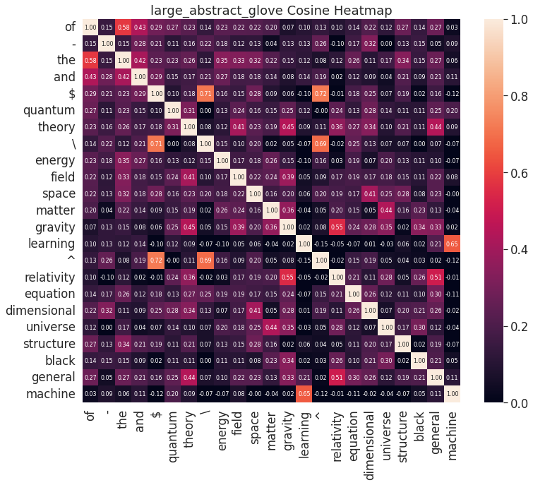
The most basic and universally-used measure for how closely related two words are is their cosine-similarity: the normalized dot-product between their associated vectors, \cos\theta_{ij}= w_i\cdot w_j / |w_i||w_j|, which measures their alignment. Below is a heatmap of the cosines between various words for one fully trained GloVe model. The entire series of heatmaps which were generated throughout the training process can alternatively be viewed here.

Some observations:

• The results look eminently reasonable and related words clearly point in similar directions. For instance, "machine" and "learning" have a large cosine with each other, but not with any other words in the set, all of which are fairly unrelated to "machine" or "learning".
• As is becoming a common theme, the algorithm picks up on a strong signal from the LaTeX equation-setting markers $, ^, and \ which necessarily appear near each other in valid LaTeX.
• It is clearly meaningful when two vectors are aligned in similar directions, but it is much less common to have significantly anti-aligned vectors whose cosine is significantly negative and the meaning of few examples in which this does happen is not very apparent. From a technical standpoint, this is entirely expected since the components of the initial embedding vectors are drawn from a standard normal distribution and are trained by enforcing w_i\cdot \tilde{w}_j\sim \ln X_{ij} (ignoring bias terms) where \ln X_{ij} is typically positive. Therefore, there does not exist an efficient mechanism for anti-aligning vectors. It would be interesting to develop a modification of GloVe in which anti-alignment also carries some semantic meaning.

Finally, two three-dimensional visualizations of the actual embedding vectors are given below. These are generated using PCA Principal Component Analysis (PCA) is another unsupervised learning algorithm. It is simply the process of finding the eigenvalues of the covariance or correlation matrix for some set of d-dimensional data points. Usually, one uses this analysis to project the full dataset onto the subspace spanned by the n eigenvectors whose corresponding eigenvalues are largest and where, typically, n \ll d, in which case PCA is used for dimensional-reduction. That is, PCA highlights the directions in feature-space along which the data varies the most, since these directions presumably represent the combinations of features which have the greatest ability to differentiate the data points from each other. and t-SNE t-Distributed Stochastic Neighbor Embedding (t-SNE) is an alternative, unsupervised, dimensional-reduction algorithm. In very rough terms, t-SNE takes the N \gg 1 original data-points {\bf x}_i, each of which are d -dimensional, and randomly initializes n-dimensional counterparts {\bf y}_i where n\in \{2, 3\} for visualization purposes. Probabilities P_{ij} and Q_{ij} are modeled using the {\bf x}_i and {\bf y}_i, respectively. P_{ij} is designed to be relatively large when the points i and j are close together in the original feature space and relatively small when they are well separated, with similar statements holding for Q_{ij}. The embedding vectors {\bf y}_i are trained by minimizing the Kullback-Leibler divergence D_{\rm KL}(P||Q) via gradient descent in the usual way.

A great post about the interpretation, use, and misuse of t-SNE can be found here. As the post points out, t-SNE primarily captures the topology of the data (if used properly) and there is no guarantee that the apparent sizes of clusters or sizes between clusters in the embedding is an accurate reflection of these properties of the original data. The host of subtleties illustrated in this post should make one extremely wary of reading too much into single t-SNE plots. respectively. The full timeline of these visualizations throughout training can be found for PCA here and for t-SNE here.