Note: The Jupyter/Colab notebooks relevant to this post are
here on my GitHub page.
My pytorch_lightning implementation of a basic feed-forward network for one-hot
encoded text (of which logistic regression is a limit)
can be
found here.
Starting Simple
There are advantages to starting a project by creating some simple models, rather than immediately diving in to
more complicated ones:
Simple models provide a baseline for later comparison and can be surprisingly effective (as in the present
case).
Simple models are often much easier to interpret. This can be useful for revealing issues in the raw data itself
or in its processing, in addition to the intrinsic appeal of interpretability.
Below I detail the results of applying logistic regression and a Random Forest to character-level, one-hot encoded
arXiv/viXra title data.
Logistic Regression
The simplest version of a fully-connected model for text analysis is the following. After one-hot encoding the
titles, all of which are padded or truncated to a fixed length, seq_len, each
data
point is a (seq_len, chars)-shaped tensor, with
chars the number of unique characters used in the encoding (see the Data post).
The resulting tensor can then be flattened into a vector
There are various differences in the tensor/array conventions and terminology used in physics and ML. In
particular, what physicists would call a D-dimensional vector \vec{v} whose
components are v_{i} with a single index i\in\{0,\ldots, D-1\}, is often
represented to in ML circles as a (1, D)- or
(D, 1)-shaped tensor (in numpy/pytorch
language) with a singleton dimension explicitly noted, meaning that they are really tensors of
the form v_{ij} or v_{ji} with i as above and
j\in\{0\}, strictly speaking (vectors which truly only have a single index can also be created, and
are denoted as being
(D, )-shaped, but these other options seems to appear more frequently).
Tracking such information is important in ML for
broadcasting purposes and it takes a little time to get used to, if coming from the more concise physics
conventions.
\vec{t}\in \mathbb{R}^{\texttt{seq\_len}\times \texttt{chars}} and
probability that a given paper title \vec{t} is from viXra is finally modeled by
Other conventions: \cdot is used both for matrix multiplication and dot products as in
W\cdot \vec{x} or \vec{x}\cdot \vec{y}, while * represents
element-wise multiplication, also known as the Hadamard product, (A* B)_{ij}\equiv A_{ij}\times
B_{ij}. ML would benefit from greater use of the Einstein summation convention (implemented in
pytorch by einsum!
) in which the usual summation symbol is left implicit in any tensor sums over indices, as the presence of
repeated indices already implies the existence of a sum: \sum_{i,j}T_{abij}U_{cidje}\longrightarrow
T_{abij}U_{cidje}. This is often (semi-)jokingly referred to as Einstein's greatest contribution to
physics. The prevalence of Hadamard products in ML does make its use a bit more confusing in that
context, however.
Above \vec{W}\in\mathbb{R}^{\texttt{seq\_len}\times \texttt{chars}} is simply another vector (the
weights) and b
is a scalar (the bias), both of which are to be tuned by minimizing the cross-entropy loss
Given D data points belonging to C classes, respectively indexed by
\alpha \in
\{0,\ldots, D-1\} and i \in \{0,\ldots, C-1\}, and a model which assigns
corresponding class probabilities to each example q_\alpha^i, the to-be-minimized empirical
cross-entropy loss is
H_{\rm empirical}(q)\propto -\sum_\alpha \ln q_\alpha^{i(\alpha)}
where i(\alpha) is the true class-label for the \alpha-th data point. This
metric is only sensitive to how poor a model's prediction for the true class label was, the distribution of
probabilities for incorrect class labels being totally irrelevant.
H_{\rm empirical}(q) is an approximation to the cross-entropy loss H(p,q),
H(p,q)\equiv -\sum_i p_i \ln q_i\ ,
for two distributions specified by p_i and q_i. In the present context
the observed data points are assumed generated according to the p_i. Minimizing H_{\rm
empirical}(q) by tuning the parameters which determine the q_\alpha^i is equvalent
to minimizing the negative log-likelihood or empirically
estimated KL-divergence (more commonly called the
Relative Entropy in physics): D_{\rm
KL}(P||Q)=-\sum_i p_i \ln \left(q_i/p_i\right).
D_{\rm
KL}(P||Q) is often colloquially referred to as a distance-measure between two distributions, since it
vanishes if p_i=q_i\ , \forall \ i and is positive otherwise, though it does not satisfy the
other usual properties of distances. Instead, the KL-divergence is better thought of as the rate at
which one will realize their error if they mistakenly model some process using probabilities q_i
when in reality it is being generated according to probabilities p_i; see Jared Kaplan's
notes for a nice discussion on this point., as usual.
This model, known as logistic regression, can only pick up on technical data in the text and not its semantics,
since it has no means for efficiently
learning about interactions between characters at different positions in the title. Nevertheless, it performs
surprisingly well (to me, at
least), achieving \approx 70\% accuracy on the validation set! For reference, humans guessing at
garrettgoon.com/arxiv-vixra/quiz also only guess titles
sources correctly
\approx 70\% of the time. The evolution of the
confusion matrix throughout training is
below (direct
link here).
Because of the simplicity of the model, it is very easy to interpret. Every entry of \vec{W}
corresponds to a single character at a single position in the text. A positive weight indicates that having that
particular character at that specific position will push the prediction toward viXra, with the analogous result
for negative values and arXiv.
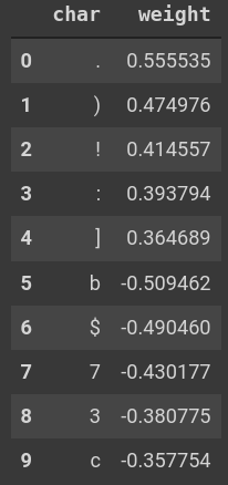
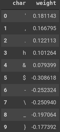
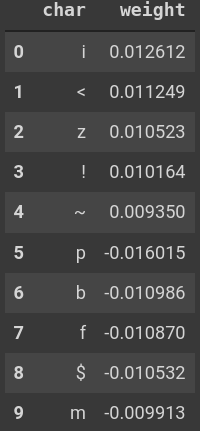
In the images below are the five most-positive and most-negative characters by weight for the last character in
all titles
(left image), for characters averaged over all possible locations in a title (middle image), and,
finally, characters in the first possible location in a title (right image). Since all titles were forced to be
of
the length seq_len = 128 with spaces inserted on the left as padding (when
necessary), the last character in each sequence should be much more
important
Taking the mean over characters, I have also verified that the largest weights by magnitude
correspond to positions near the end of titles, meaning those are the most informative locations, as one would
expect.
than the first character, and this is
clearly borne out.
Values of the trained weight vector \vec{W} for various characters corresponding to the final
character (left), the mean over all character positions (middle), and for the first character (right). The
three
signals are ordered by decreasing importance, as seen from their typical magnitudes.
The model has picked up on the fact that viXra papers are more likely to end with a period, exclamation point,
or
other punctuation marks, while arXiv papers are more likely to end with some numerical value or a dollar-sign
(presumably due to LaTeX equation setting). Averaging over all positions,
viXra
papers are more likely to have commas anywhere while most of the top arXiv markers are again associated with
LaTeX. These LaTeX signals will be a
persistent theme. The below images inspect these findings in further detail.
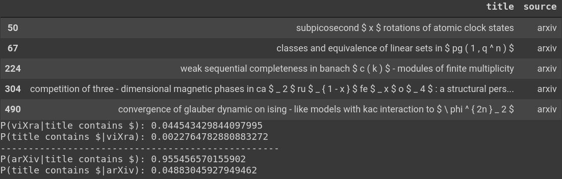
Examples of titles which contain \$ and the relevant conditional probabilities. Empirically,
a
\$ in a title indicates a \sim 96\% chance that the paper is arXiv, but only
\sim 2\% of all titles have a dollar-sign anywhere.
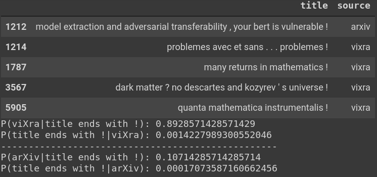
Examples of titles which end with ! and the relevant conditional probabilities. Empirically,
a
! ending a title indicates a 89\% chance that the paper is viXra, but only
a tiny fraction of all papers end with an exclamation point.
Finally, logistic regression has picked up on the fact that viXra papers tend to be shorter than arXiv ones, as
indicated by the fact that they typically have more left-padding by blank spaces when forced to be of length
seq_len = 128. In the figure below, the top plot shows the weights assigned to
blank space summed from position zero in the sequence up to the position marked on the horizontal axis. The sum
initially trends towards arXiv and flattens out position \sim 60
and then strongly reverses course towards viXra around positions \sim 75 and beyond.
Correspondingly, titles whose non-trivial content starts somewhere before this latter dividing line have
accumulated a bias towards arXiv, while those which start somewhat after this point are weighted towards viXra.
Not
coincidentally,
the scales of these inflection points coincide with the mean start positions for arXiv and viXra titles, se the
vertical lines in the plot show.
The bottom plot demonstrates similar behavior for the average non-blank-space weights summed from the end of the
sequence
to a given position.
In the next section, we will again see that character length is one of the primary predictors for a title's
origin.
Top plot: the cumulative sum of weights corresponding to all blank spaces, starting from position 0, described in more detail above. Bottom plot: the cumulative sum of the mean of
all non-blank-space weights, starting from position 128. Since all titles end
with non-blank characters, the sum is non-informative towards the end of the sequence. As the title length
increases and one moves to the left of the plot, the sum increasingly indicates an arXiv paper.
Random Forest
I used a Random Forest
In brief, a Random Forest classifier works by generating a large number of decision trees which are each trained
using a
randomly selected set of training examples and a randomly selected subset of data features. The conditions for
generating a terminating leaf
are controlled by various hyperparameters, such as the maximum depth of the tree or number of training examples
remaining post-split. In a binary classification context, the
Random Forest then makes a prediction for a new data
point by passing it through all of the collected trees and taking a majority vote based on the various leaves
the data point settles in.
The random selection of data points and features for each tree and the averaging procedure at inference time
are the key features which decorrelate trees and combat variance.
as a second baseline model. In order to facilitate training, I also
performed a modest amount of feature engineering such as computing the frequency with which
various forms of punctuation appear in titles and the length of the title's longest word, resulting in 64 total
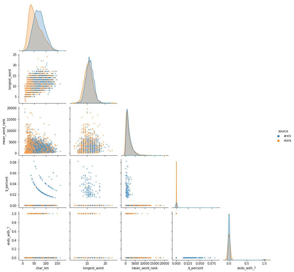
features. See the figure below for the data distributions along some particular engineered feature-directions.
The ultimate model (which only uses ten of the 64 features, discussed below) achieved approximately the same
validation-set
performance as logistic regression: \approx 70\%
accuracy.
A corner plot of a few features used by the Random Forest. mean_word_rank
is
the average rank of all words in each title, as computed from the ranks of how common each word is in the
training set.
Sixty-four features is too many to be useful for a simple quick-and-dirty baseline. Apart from some quantitative
benchmarks, one also wants a greater understanding of what features are important in distinguishing arXiv
papers from viXra, and most of the 64 are not.
There exist two common methods for quantifying the importance of different features in a Random Forest:
Gini-Impurity-Based Importance: in sklearn, the split-points in trees
are determined by maximizing Gini Impurity
The Gini Impurity of a set of data points belonging to C classes, indexed by i
\in\{0,\ldots, C-1\}, is
given by the probability of misclassifying a randomly chosen data point when using a simple strategy in
which
you
randomly guess which class the point belongs to in proportion to the relative class populations of the whole
set. That is, if p_i is the probability of drawing from class i, then
the
impurity is given by
I_G = \sum_i P({\rm misclassify}|c_i)P(c_i) =\sum_i (1-p_i)p_i\ .
If the
data set only has elements from one class, then I_G is minimized at zero, while an
equally-balanced dataset has maximal I_G. A Random Forest strives to make splits such that
all examples which end up in a leaf of a tree belong to the same class, which is equivalent to minimizing
I_G.
decrease by default. By creating a weighted average of the Gini Impurity decrease achieved by
every split
in every tree per split-upon-feature, one estimates the relative importance of all features.
sklearn implements this method via feature_importances_.
Permutation-Based Importance: a more computationally-expensive metric for assessing feature importance is
to calculate the drop in performance which comes from randomly shuffling the values for a single feature in some
validation set, repeating this process for each feature.
sklearn implements this method via permutation_importance
The Gini-Impurity-based method has been criticized as overestimating the importance of
features which allow for many possible choices of split-points. As done in the preceding link, this effect can be
seen by adding a test-feature which consists solely of randomly generated numbers drawn from a simple Gaussian.
Adding such a feature to the
data and computing feature importances as above, the Gini method ranked this
random feature as the 17th most-important feature, while permutation importance
more-reasonably has it
ranked dead-last: 65 of 65. See the plot of permutation-based importances below.
The losses in accuracy when different feature dimensions are shuffled. Multiple shuffle-iterations are performed
for each feature and the error bars come from the standard deviation across shuffles. Shuffling the
random feature improves performance, presumably since it washes out the
unwanted effects created by training on this uninformative column in the first place.
There are clearly many uninformative features. As a quick-and-dirty contraction of the model, I re-trained the
Random Forest on the top-ten
Reducing the number of features slightly increased the performance of the model. In general, one should
also carefully consider the correlations between different features before winnowing down the elements which are
fed into a Random Forest, but taking the top-ten was good-enough for present purposes.
features per the above chart, resulting in the more-focused importances plot below.
As found in the logistic regression model, many of the most-informative markers regarded the use of punctuation
marks and the overall length of the title. Unlike logistic regression, the Random Forest also had access to how
common the words in each title were ( mean_word_rank), which also carried
significant meaning, as one might have suspected.
Permutation-based importances for the ten most-important columns.
Lastly, it can be informative to get an inside-view of what is going on in the various trees which comprise a
Random Forest.
The dtreeviz package
is a useful tool for this purpose. There exist methods for visualizing how groups of data or individual
titles filter through the leaves of the tree. An example of the path that one of my own papers takes when
traversing a single tree is below. A visualization of 500 validation-set samples being filtered into the leaves
of the same tree is a bit more unwieldy, but can be found here.
An (incorrect) prediction-path for one of my papers (
Gauged Galileons From Branes) from one tree in the Random Forest, as visualized by dtreeviz. The yellow bars indicate the distribution of
all twenty of my papers, while the orange arrow points to the statistics of
Gauged Galileons From Branes and the black arrow marks the split-points.
Performance on My Papers
I, of course, have to check the model performance on
my own papers (which are all arXiv), which I will do for each model in this series of posts.
The results aren't great for these baselines! Both models only classify half of my papers correctly. As seen in
the figures below, there
is a clear trend for longer titles to be predicted as arXiv and shorter ones as viXra, as expected from the
above. This might be expected, given the lack of
LaTeX and related technical markers in the titles of my
papers.
Probabilities that each of my titles are viXra, as predicted by the logistic regression model.
Probabilities that each of my titles are viXra, as predicted by the Random Forest, as estimated by computing
the
mean prediction over all trees in the forest.
Acknowledgments
Thank you to the Distill team
for making their
article template publicly
available. Discussions with Matt Malloy and Rami Vanguri for gaining an intuition for the various
hyperparameters used in a Random Forest.
Additional Links
Jeremy Howard has great videos on the practicalities of (and some theory behind) Random Forests, such as here
and here.
Notes on Random Forest hyperparameter tuning from his fastai course can
be found here.
Random forests are also useful for analyzing the performance other ML architectures. Weights and Biases (used
extensively for
this project, see the Workflow post) uses Random Forests to estimate the
importance of various
hyperparameters across model training runs via
the permutation-based method detailed above.
All Project Posts
Links to all posts in this series.
Note: all code for this project can be found on my GitHub page.