arXiv/viXra - Simple Recurrent Models

Note: The Jupyter/Colab notebooks relevant to this post are here on my GitHub page. Mypytorch_lightning implementation of the simple RNNs considered in this post can be found here.

Sequential Information

A central limitation of the baseline models considered previously is that they have no means of efficiently using the information inherent to the ordering of the text. For instance, one would expect that the logistic regression and random forest models would perform just about as well Apart from some specific minor degradations, such as the weakening of the signal which arises when a title ends in a punctuation mark (an uncommon, but strong, viXra signal). if we were to shuffle around the words in each title.

Recurrent Neural Networks (RNNs) are the basic architecture which attempts to capture the information in the relative ordering of inputs. I briefly review their properties below, some details of their implementation in pytorch, and examine their performance on the arXiv/viXra data and on my own papers.

RNNs, Briefly

General Structure

RNNs are relevant when our input data forms an ordered series x_t, t\in\{1,\ldots, \texttt{seq\_len}\}. In the context of arXiv/viXra, the x_t would be (tensorial representations of) the individual characters or words in a title with t indexing the position of these elements in the title.

The inputs x_t are consumed sequentially and are used to update an internal state of the RNN, h_t, a hidden or latent variable. The update step also takes into account the form of the previous hidden state, h_{t-1}, and this pattern continues on and on such that h_t contains information from all previous inputs and hidden states all the way back to the initial The initial hidden state h_0 is often taken to be a tensor filled with zeros. This is the default behavior pytorch, for instance. However, it is generally beneficial in Machine Learning to allow the model to figure out its own best parameters, when possible, and the best practice is to promote the initial state to a learnable parameter; see, e.g., Hinton's RNN presentation, slide 14.

It is easy enough to implement this in a pytorch model (minimal sketch): class DynamicInitialHiddenRNN(nn.Module):   """Adds a learnable initial hidden state to the vanilla torch RNN.   """   def __init__(self, input_size: int, hidden_size: int):     super().__init__()     self.rnn = nn.RNN(input_size, hidden_size, batch_first=True)     # Initialize the hidden state randomly.     self.initial_hidden = nn.Parameter(torch.randn(1, 1, hidden_size))   def forward(self, inputs: Tensor, hidden: Optional[Tensor] = None) -> Tuple[Tensor, Tensor]:     if hidden is None:       hidden = self.initial_hidden       # Expand hidden to match batch size and ensure contiguous.       batch_size = inputs.shape[0]       hidden = hidden.expand(-1, batch_size, -1).contiguous()     output, hidden = self.rnn(inputs, hidden)     return output, hidden h_0. This long chain of dependencies can create difficulties in training For very long sequences of length-T, it is common to process the sequence in length- n\ll T chunks (with n determined by practical considerations), performing backpropagation only over these subsequences and passing the resulting final hidden state h_n along to be used as the initial state for the next n terms. More specifically, the computational graph is reset after each sub-sequence via calls of the form hidden.detach() in pytorch, since memory constraints forbid performing backprop over the full, length- T sequence. This procedure goes by the name of truncated backpropagation through time (TBPTT).

In pytorch_lightning TBPTT is performed automatically and there is no need for manual .detach() calls if an self.truncated_bptt_steps attribute is set for architecture (a pl.LightningModule subclass), though I found the whole process somewhat underdocumented. After every training step, pl extracts the hidden states of the architecture and recursively detaches them in the process. In my experience, getting TBPTT to function in the expected manner also requires overwriting the tbptt_split_batch method with a custom implementation, as the default seems to make some curious assumptions .

The hidden states h_t are also the outputs of the entire network, one or more of which are then used for further purposes. In the context of arXiv/viXra text classificaiton, the simplest use would be to take the final hidden state h_{\texttt{seq\_len}}, which carries information about the entire sequence, and feed this into a fully connected layer and sigmoid function to predict the classification probabilities of a given title.

A Specific Architecture: Gated Recurrent Units

I used Gated Recurrent Units (GRUs) as the recurrent layers The other basic recurrent architectures which are commonly seen are so-called vanilla RNNs and long short-term memory (LSTM) layers. Simple trials demonstrated that GRUs performed similarly well on arXiv/viXra classification to LSTMs (both architectures faring better than vanilla RNNs, as expected), while training faster and being more compact, as they only require one latent variable in contrast to the two needed for LSTMs. See nn.RNN , nn.LSTM , and nn.GRU for the pytorch implementations of these architectures. in the arXiv/viXra models. GRUs process an input x_t via the following steps All of the x_t are generally encoded in three-dimensional tensors shaped as in (batch_size, seq_len, input_size), assuming a pytorch, batch_first = True type implementation (assumed throughout). E.g. for a batch of 50 one-hot encoded text samples, each 100 characters long and which only use lower case characters a-z, the x_t would be (50, 100, 26) -shaped. Similarly, all of the h_t are ensconced in a (b * num_layers, batch_size, hidden_size)-shaped output tensor where hidden_size is the length of the hidden state vector, num_layers is the number of stacked recurrent layers, and b = 2 if bidirectional else 1 doubles the size of the hidden state if the architecture is also bidirectional; see below. The batch dimensions are processed in parallel in the steps outlined below. Indices on x_t, h_t will generally be suppressed, as in the above. I have also compressed the separate b_{iz} and b_{hz} biases of the pytorch nn.GRU implementation into a single b_z vector for brevity and similar for b_r. :

• Use x_t and the preceding hidden state h_{t-1} to determine what fraction (element-wise) of h_{t-1} to hold onto and include in the updated state h_{t}. The fraction $z_t$ is determined through the usual process of using weight-matrices (W), bias-vectors (b ), and a sigmoid function \sigma(x) , z_t \equiv \sigma\left(W_{iz} \cdot x_t +W_{hz}\cdot h_{t-1} +b_z\right)\ , such that the updated state will be of the form h_t= z_t * h_{t-1}+\ldots
• Use x_t and the preceding hidden state h_{t-1} to determine what new information from x_t to include in the updated state h_{t}. This new data n_t is determined through a similar process of using weights, biases, and non-linearities, applied pointwise: n_t \equiv \tanh\left(W_{in}\cdot x_t + b_{in} +r_t * \left(W_{hn}\cdot h_{t-1}+b_{hn}\right)\right) where r_t is defined similarly to z_t r_t \equiv \sigma\left(W_{ir} \cdot x_t +W_{hr}\cdot h_{t-1} +b_r\right)\ .
• The fully updated hidden state is a weighted sum This weighted-sum update step between h_t and h_{t-1} is one of the central advantages of GRUs (and LSTMs) over the vanilla RNN architecture in which the update step is instead of the form h_t = \tanh\left(W_{ih}\cdot x_t +W_{hh}\cdot h_{t-1} + b_h\right). To see one reason why, consider the limit in which the data has provided a very strong signal at some time-step t with all later data points being relatively uninformative. In this case, the architecture would perform best by holding onto the information in the current hidden state h_t, using its parameters to maintain h_{t'} \approx h_t for all t'\ge t. The GRU could accomplish this relatively easily by ensuring the pre-activations (arguments of \sigma) of the so-called update gate z_t are large and positive, such that z_t\approx {\bf 1} is nearly the identity and thereby propagating forward the current hidden state relatively unscathed: h_{t}\approx h_{t-1}. Accomplishing the same means in the vanilla RNN is much more difficult, as one would need to choose the weights and biases such that h_{t} = \tanh\left(W_{ih}\cdot x_t +W_{hh}\cdot h_{t-1} + b_h\right)\approx h_{t-1} which is a far-tougher balancing act. In particular, even if one made the optimistic assumptions that the architecture could learn to push the weights and biases into the regime in which \tanh is approximately linear and the \sim W_{ih}, b_h terms contribute negligibly, such that h_t \approx W_{hh}\cdot h_{t-1}, then achieving the desired goal would still require carefully tuning W_{hh} so that it nearly acts on h_{t-1} as the identity. And even if this were accomplished so that hidden states at neighboring time-steps were approximately equal, states separated by n time-steps still diverge exponentially, scaling like the largest eigenvalue of W_{hh} ( \lambda_{\rm max}) to the n-th power: h_{t+n}\sim \lambda_{\rm max}^n h_t. This type of scaling is a general problem for RNNs, regardless of whether they are attempting to hold onto the current hidden state, known as the vanishing and exploding gradient problem. The weighted-sum update step of the GRU helps ameliorate this issue, though it does not resolve it entirely. of the previous hidden state h_{t-1} and the new information n_t: h_t = (1 - z_t)* n_t + z_t * h_{t-1}

The weights W and biases b are the learnable parameters of the model. The set of h_t's for allt form the output of the GRU.

Bells and Whistles: More Layers and Directions

Finally, one could increase the depth of the RNN architecture by stacking multiple such layers and could also process the inputs x_t in both the forward and backwards directions, resulting in a bidirectional architecture.

Both features are essentially what they sound like, though the details are important.

• Stacking M RNNs leads to multiple hidden states: h_t \longrightarrow h_t^i, i \in\{0, \ldots, N-1\}, one per layer. While the x_t are still the inputs for the first i=0 layer, subsequent layers with i>0 process the hidden state of the preceding layer (h^{i-1}_t) as their input. The outputs of the stacked RNN are the hidden states of the final layer across all time-steps: h^{N-1}_t .
• Bidirectional RNNs process the inputs forwards and backwards, with independent weights and biases used for each pass. This is desirable in contexts such as arXiv/viXra classification, since the passes in the two directions capture different contextual information. In pytorch, the outputs of a bidirectional architecture come from concatenating the hidden states of the two passes together I found the concatenation step a little under-documented. Theoutput tensor is (batch_size, seq_len, 2 * hidden_size)-shaped, but it is not clear from the documentation what the entry at time-step t (output[:, t]) corresponds to, precisely. Presumably (and correctly), the first half of the output (output[:, t, :hidden_size]) is the hidden state generated after stepping through the first t inputs (x[:, :t]) in the forward direction. But do the entries output[:, t, hidden_size:] corresponding the backwards direction arise from stepping backwards through the final t entries of the input or through all entries from the end of the sequence all the way back to entry t? x[:, -t:] or x[:, t:]?
  
  The answer is the latter: output[:, t] contains information from processing the first t input entries in the forwards direction and the final seq_len - t entries in the backwards direction. One can ask similar questions regarding the hidden tensor returned by the RNN and, thankfully, these are what one would expect: they are the final hidden states which arise from a forward pass and a backward pass, concatenated into a (2, seq_len, hidden_size)-shaped tensor. These statements can be verified (following this nice post) by creating a bidirectional RNN, two single-direction RNNs which have their weights tied to the bidirectional one, and comparing theoutput andhidden tensors of each as they run through a sequence in the relevant direction(s): # Create three simple GRUs, one of which is bi-directional. forward_gru = nn.GRU(input_size=1, hidden_size=1, batch_first=True) backward_gru = nn.GRU(input_size=1, hidden_size=1, batch_first=True) bi_gru = nn.GRU(input_size=1, hidden_size=1, batch_first=True, bidirectional=True) # Tie their weights together. for name, p in forward_gru.named_parameters():   getattr(forward_gru, name).data = getattr(bi_gru, name).data   getattr(backward_gru, name).data = getattr(bi_gru, name + '_reverse').data # Pass inputs and reversed inputs as relevant into the RNNs. rand_input = torch.randn(1, 3, 1) rand_input_flip = rand_input.flip(1) forward_gru_output, forward_gru_hidden = forward_gru(rand_input) backward_gru_output, backward_gru_hidden = backward_gru(rand_input_flip) backward_gru_output_flip = backward_gru_output.flip(1) bi_gru_output, bi_gru_hidden = bi_gru(rand_input) # The below vanishes. forward_backward_output = torch.cat((forward_gru_output, backward_gru_output_flip), dim=-1) output_difference = forward_backward_output - bi_gru_output torch.testing.assert_close(output_difference, torch.zeros_like(output_difference)) forward_backward_hidden = torch.cat((forward_gru_hidden, backward_gru_hidden), dim=0) hidden_difference = forward_backward_hidden - bi_gru_hidden torch.testing.assert_close(hidden_difference, torch.zeros_like(hidden_difference))
  
  Importantly, this means that if we wanted to use the hidden states which contain information from having seen the entire sequence in both directions, we would need to extract output[:, -1, :hidden_size] and output[:, 0, hidden_size:], not simply the final entry output[:, -1]. .

RNNs for arXiv/viXra

Sticking to the theme of starting simple, I analyze the performance of single-layer, uni-directional GRUs on arXiv/viXra title data Experiments with additional layers and bidirectionality only led to modest improvements upon the results reported below. .

Character- or Word-Level?

One needs to decide how exactly to encode the text as a series of tensors x_t. The natural options are as follows:

• One-Hot Encode: The simplest option is to let each time-step correspond to a single character and represent each such character as a vector pointing in some cardinal direction That is, if we index each of the possible C, say, characters by an integer c \in \{0, \ldots, C-1\}, then denoting the character appearing at time-step t by c_t , one-hot-encoding corresponds to taking x_t^i = \delta^i_{c_t} with i the vector index. The x_t are then (batch_size, seq_len, C)-shaped. pytorch has a built-in F.one_hot method for one-hot encoding text given an chars tensor holding character indices, but it's a nice exercise in using vectorized code to figure out how one would perform the encoding manually.
  
  When chars is a simple one-dimensional, (seq_len, )-shaped vector such that chars[t] corresponds to the character index at the t-th position in the text, then the associated one_hot tensor of shape (seq_len, C) can be generated by creating a zero-tensor of this same shape and then inserting ones at all appropriate locations, as in: # Use a random character sequence. chars = torch.randint(C, (seq_len, )) one_hot = torch.zeros(*chars.shape, C) one_hot[torch.arange(*chars.shape), chars] = 1.
  When chars instead has a batch dimension and is of shape (batch_size, seq_len), such that chars[b, t] corresponds to the character index at the t-th position in the text in the b-th document in the batch, one can instead use the .scatter_ method to insert ones into the appropriately shaped zero tensor in a vectorized manner: # Use a random character sequence. chars = torch.randint(C, (batch_size, seq_len)) one_hot = torch.zeros(*chars.shape, C) one_hot.scatter_(dim=-1, index=chars.unsqueeze(-1), src=torch.ones_like(one_hot)) which is essentially what F.one_hot is doing under the hood. .
• Embeddings: Alternatively, one could let each time-step correspond to a single word Or other series of characters separated from others by white space, per the details of text-normalization. We will refer to them all as "words", for simplicity. in the text. There are commonly V\sim \mathcal{O}(10 ^5) or more unique words in a corpus' vocabulary, as opposed to C\sim \mathcal{O}(10 ^2) characters, making a one-hot encoding infeasible. Instead, we can assign each word to a vector living in some embedding_dim \ll V-sized vector space, with the components of each vector randomly initialized. The vector components are learnable parameters which mutate upon training.

I use both options. For embeddings, there are various choices to make. One has to choose both the dimension of the embedding space The embeddings are stored in a (V, embedding_dim)-shaped matrix E . Empirically, choosing embedding_dim \sim \mathcal{O}(10^2) apparently works well on most NLP tasks and choosing a dimension much larger than this only has a weak effect on performance, if any. There has been progress in understanding this finding on a theoretical level by analyzing the so-called Parwise Inner Product (PIP) loss which is the Frobenius norm of the difference between the inner-products along the embedding_dim -sized dimension of two differnent embedding matrices: {\rm Loss} = || E_1 \cdot E_1^T - E_2 \cdot E_2^T|| This loss is a measure of the inherent similarity between the two embeddings since, for instance, if E_1 and E_2 only differed by a rotation in the embedding space, then the loss would vanish. The referenced paper finds a bias-variance decomposition for the loss between the ideal ("oracle") embedding matrix, E , and a estimator thereof, \hat{E}, and demonstrates how these contributions grow and shrink as the embedding_dim of \hat{E} varies with respect to that of E. , denoted by embedding_dim, and one might also choose to only work with a subset of the vocabulary, as the vast majority of the words in a corpus are captured in a tiny fraction of the vocabulary, a general phenomenon known as Zipf's law. See the plot below. I set embedding_dim = 256 and work with the whole V\sim \mathcal{O}(2 \times 10 ^4)-sized vocabulary for arXiv/viXra titles.

Architecture Details

The recurrent models are all fairly simple: the GRU consumes the one-hot-encoded or embedded text as inputs and the ensuing hidden states (which are optionally first passed through a dropout layer) are fed into a single fully-connected layer to predict a single number, the probability that a given title comes from a viXra paper. I use hidden_size = 512 for all models.

The python code for the relevant nn.LightningModule subclasses can be found in the arxiv_vixra_models package. The code also accommodates the additional bells and whistles listed above and further features not detailed here.

An important choice is precisely what data from the GRU hidden states is passed to the feed-forward layers. While we could pass in only the hidden state from the final time step, since that is the unique state which has seen the entire title text, this choice poses the risk of missing out on important information that may have appeared early on in the title but which has faded out of the hidden state with time. So, instead of passing in this final time-step (output[:, -1]), one might instead use the maximum across all time steps for each hidden_size dimension (output.max(dim=1)), the similar mean across all time-steps (output.mean(dim=1)), or even concatenate all three options together, as suggested in the ULMFiT paper. Why be so rigid in choosing which portions of the hidden state to pass to the feed-forward network? Why not allow the architecture to dynamically choose which parts of the text to focus on by, say, using more finely-weighted averages of the different time-steps? Such an idea is a simple version of an attention mechanism, which will be explored in a later post.

The arxiv_vixra_models code accommodates each of these options and empirically the max option tended to perform best, though difference between the strategies were not large.

Performance and Interpretation

Validation Set

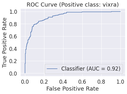
The one-hot and embedding-space recurrent architectures both achieved \approx 83\% accuracy on the validation data, which is significantly better than the \mathcal{O}(70\%) peformance of the simple baseline models discussed previously. Of the two models, the embedding-space architecture performed very slightly better. The ROC curve Receiver Operating Characteristic (ROC) curves plot the true-positive-rate (often called precision) on the y-axis and false-positive-rate on the x-axis as the threshold for what constitutes a positive prediction is varied. (In the context of arXiv/viXra, P({\rm pred. = viXra}|{\rm source =viXra}) is the vertical and P({\rm pred. = viXra}|{\rm source =arXiv}) is the horizontal.) By threshold, I am referring to the fact that classification models are assigning a score to every example and this score is used to set the prediction boundary. In the canonical case, the score is given by the logits and one usually declares that positive and negative logits correspond to a positive and negative predictions, respectively, but one could also consider moving this boundary away from zero. As the threshold is varied, the relative true- and false-positive-rates change, generating the below curve. The top-right corner corresponds to sending the threshold to -\infty (classifying all positive cases correctly, but also generating many false-positives) and the bottom-left corner is the opposite limit.

Denoting the abstract score assigned to an example by s, the positive and negative examples belong to separate distributions, \rho_1(s) and \rho_0(s), respectively. The area under the curve (AUC) has a lovely, precise meaning: it is the probability that the score the model assigns to a randomly chosen positive example will be higher than that of a randomly chosen negative example, {\rm AUC} = \int_{-\infty}^{\infty}{\rm d} s_1{\rm d} s_0\,\theta(s_1 - s_0) \rho_1(s_1)\rho_0(s_0)= P[S_1 \ge S_0]\ . for the embedding model can be found below. A disadvantage of the present architectures relative to the baseline models, however, is that they are much more opaque. What, exactly, is the recurrent architecture picking up on that was missed by the simple baselines?

Interpretation

The simplicity of the present models allows us to see a glimpse of what is going on, though it is hard to draw any very precise conclusions. In particular, the single number that our model predicts (the probability that a given title is from a viXra paper) arises from a dot-product between the final dimension of the relevant components of the GRU output tensor and an appropriately shaped vector. For example, if we only feed the hidden states from the final GRU time-step into the fully connected layer, then this (batch_size, 512)-shaped tensor is turned into logits by taking a dot product with a (1, 512)-shaped weight vectorw and adding the scalar bias b to the result.

This means that by re-scaling the GRU hidden states by the appropriate weights and biases, we can get a direct view of the logits More precisely, if output is (batch_size, seq_len, hidden_size)-shaped hidden state tensor of the GRU model, wherehidden_size = 512, then the plot below shows a handful of entries along the batch_size dimension of logits_output for a particular slice of neurons along the hidden_size dimension with logits_output defined as in (sketch): w, b = model.weight, model.bias logits_output = output * w + b / output.shape[-1] When the model uses only the final time-slice to make viXra-probability predictions, as in thtensor could be computed ase plot below, thenlogits_output is related to the (batch_size, )-shaped probs probability tensor via last_step_logits = logits_output.sum(dim=-1)[:, -1] probs = last_step_logits.sigmoid() . While other strategies perform better, the case where one makes predictions based on the final hidden time step is easiest to interpret. The below plot shows how various, re-scaled hidden-state neurons of one such model are pushed towards a viXra signal (light) or arXiv signal (dark) as they step through three titles from my papers. The logits in each case would come from summing up the final (rightmost) column and adding this to the similar sum of neurons not shown in the plot.

Though the evolution in the model's prediction can be clearly seen in each case, it's difficult to interpret what any individual neuron is looking for (nor should such human-interpretable behavior be expected). There are some intriguing signs, but most seem to fall apart under scrutiny. For instance, the bright streak in the top image could plausibly be attuned to title length as its viXra signal grows as it sees more and more padding and terminates in a moderate viXra-leaning signal for this very short title. However, these same neurons terminate in a slightly arXiv-leaning signal for the similarly-short middle example and in the final image the neuron whiplashes back and forth upon encountering text and terminates in a moderate viXra signal for this much-longer title. Inconclusive.

My Papers

Finally, I examine the architecture's performance on my own papers. These models performed much better than the baselines when predicting the source of my own papers, thankfully, classifying 17- and 18-out-of-20 correctly for the word-embedding and one-hot models, respectively. See the figures below.

There is no longer an obvious correlation between title-length and viXra-probability, as there was for the baseline model predictions.